When evaluating an integral on a grid, the finite resolution thereof can affect the accuracy of the result. In the context of atomistic simulation, this is because a slight change in nuclear coordinates will affect the mapping on the grid.
For smooth properties like the electron density, there is a workaround. Akin to Simpson’s rule where polynomials are fitted to the grid points first and then the piecewise defined polynomials are integrated, a refinement of the grid can achieve the similar improvements in integration.
While the smart way would be to not build the grid in memory but rather integrate as you go, the following is a simple and reasonably fast implementation by explicit grid refinement in python.
import numpy as np
import scipy.ndimage as snd
import matplotlib.pyplot as plt

# generate data to operate on
data = np.arange(16).reshape(4, 4).astype(np.float)
data[0, 3] = 0
data[0, 1:3] = 5

# visualisation only
f, axs = plt.subplots(1, 2, dpi=300)
ax_2d, ax_scan = axs
ax_2d.imshow(data)

# refine grid: build grid
X, Y = np.mgrid[0:3:50j, 0:3:50j]
positions = np.vstack([X.ravel(), Y.ravel()])

for order in range(6):
    # refine grid: fit splines, re-evaluate function on grid
    a = snd.map_coordinates(data, positions, mode='nearest', order=order)
    ax_scan.plot(np.linspace(0, 3, 50), a[:50], label='Order %d' % order)
ax_scan.legend()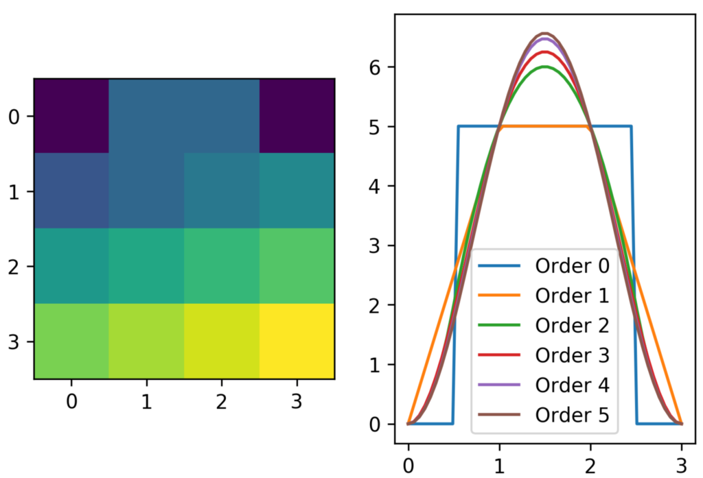
The parameter order specifies the interpolation order. You’ll need to set it to match your computational problem. This solution generalizes to arbitrary dimensions, even though the number of gridpoints scales unfavourably.